Polar Coordinates

Polar coordinates offer another way to graph equations that look like circles, spirals, ellipses, clover leaves, and any other shape with more than one point in a vertical position. The polar graph uses two elements to locate a point. First we choose an angle, $\theta$, proceeding from the horizontal axis (the non-negative $x$-axis) in a counter clockwise direction. Once we have gone around the origin $\theta$ degrees, then we move a length, $r$, in the $\theta$ direction. That defines the point, with elements $(r,\theta)$. Usually, we either develop an equation in polar coordinates, or in a few cases we might be given an equation in polar coordinates. In a school setting, about the only thing that is ever done with this system is to convert between Cartesian and polar coordinates, going either way. Most graphing calculators and CAS programs are capable of graphing polar equations, but it is greatly under-utilized.

The original polar graph was a series of concentric circles, each of radius $r$. Angle $\theta$, going from $0$ to $2\pi,$ is the angle counted counter-clockwise from the positive $x$-axis. In making a polar plot, it is usually safe to assume that the domain for $\theta$ is $0\le\theta\le2\pi$. In current CAS programs, the polar plots are actually placed onto Cartesian coordinates internally using the transformation $x=r\cdot \cos(\theta)$ and $y=r\cdot \sin(\theta)$. For example, SAGE does polar plots using that transformation, but when giving SAGE the equation, the input is given as $r(\theta)$. Since the only thing that SAGE will polar plot is equations, if we want some points or lines plotted, they can be put onto the same graph using Cartesian coordinates with user conversion from polar to Cartesian.

The first equation that we consider in polar coordinates is $r=a$, where $a$ is a constant. Right away we see that there is no $\theta$. This is the same idea that we would have with a Cartesian equation that was missing an $x$. For example $y=a$. In the polar equation we can say that no matter what value $\theta$ takes, that the $r$ distance will be $a$. You should be able to imagine that we will create a circle.

The second equation that we will propose is $$r=a^{2}sin(2\theta)\quad 0\le\theta\le 2\pi \tag{EQ1} \label{EQ1}$$ with $a=3$. I have plotted this in Figure 1.

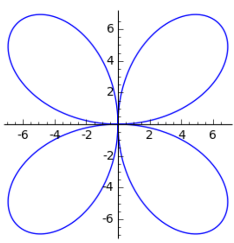
We can convert \eqref{EQ1} to Cartesian but it isn't pretty, equation $\eqref{EQ2}$, and it is difficult to plot even for a CAS that can handle an implicit equation. Using the implicit plot feature of SAGE, it has to be plotted twice, once with the positive radical and once with the negative radical. $$x^{2}+y^{2}=2a^{2}\frac{x\cdot y}{\pm\sqrt{x^{2}+y^{2}}} \tag{EQ2} \label{EQ2}$$ There are many equations, like equation $\eqref{EQ1}$ that are considerably less complex when written in polar coordinates. We will take the example of an ellipse, but first we need to show how to convert between Cartesian and Polar coordinates.